


Kalman Filter is an amazing tool in order to estimate the predicted value.
What is Kalman Filter?
Kalman Filter is an iterative mathematical process that uses a set of equations and consecutive data inputs to quickly estimate the true value, velocity, position, etc of the object being measured when the measured values contain unpredicted or random error or variation.
The reason for doing this is that we can quickly estimate the true value. Let's say for example if we want to estimate some value from a distribution of data, then we have to collect a whole set of data then calculate the average value of data from the distribution, and that average value has to be very close to the actual true value, whereas, in case of Kalman Filter, it does not have to wait for the whole set of data inputs from the distribution, it just takes some few of the inputs understanding the uncertainty or variation of those data inputs to calculate the estimate of true value.
Kalman Filter is used in RADAR technology or GPS tracking satellites, we need to know the position of the target we are tracking.
Flowchart of Kalman Filter
Below is an example flowchart of the working of the Kalman Filter.
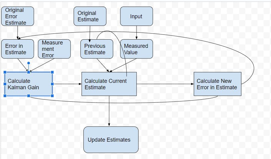
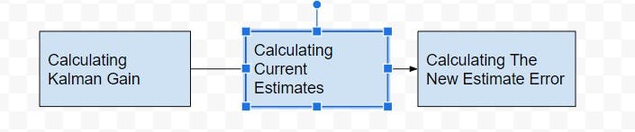
There are three main calculations that need to be done:
Calculate Kalman Gain
Calculate Current Estimates
Recalculate the New Error in Estimate
These calculations are used iteratively to estimate true value/position/velocity.
Kalman Gain
Kalman Gain helps us to determine how much of the new measurement is used in order to update the new estimate.
Kalman Gain is the ratio of the Error in estimate divided by the sum of error in estimate and error in measurement.
$$KG = \frac{E_{st}}{E_{est}+E_{mea}}$$
$$where KG = Kalman Gain, E_{est} = Error in estimate, E_{mea} = Error in measurement$$
Then, Kalman Gain is used while estimating current estimates
$$EST_{t} = EST_{t-1} + KG * (MEA - EST_{t-1})$$
$$Current Estimate = Est_{t}, Previous Estimate = Est_{t-1}$$
If Kalman Gain is very large i.e. very close to 1 then we can say that the measurements are accurate and estimates are unstable, so if the error in measurements is minimal, we do want to contribute much of the update to the estimate by the measure that we took.
But if the Kalman Gain is very small which means that the error in measurement is very large relative to the error in the estimate, since the measurement has a significant error in it, so I do not want to put much more weightage on it, so if Kalman Gain is very close to zero which means estimates are stable while measurements are inaccurate, and we want to put more weight in current and the previous estimates to update the current estimates and want to put less weight on the measured value, so we are only adding a small portion of
$$MEA - EST_{t-1}$$
Three calculations of Kalman Filter
$$Kalman Gain = KG, Error in Estimate = E_{est}, Error in Measurement = E_{mea}$$
$$Current Estimate = EST_{t}, Previous Estimate = EST_{t-1}$$
$$KG = \frac{E_{EST}}{E_{EST} + E_{MEA}}$$
First, Kalman Gain is calculated using equation 1,
$$EST_{t} = EST_{t-1} + KG * ( MEA - EST_{t-1})$$
After calculating Kalman Gain, we have to calculate the current estimates, using previous estimates, measurement value, and Kalman gain as inputs.
$$E_{EST_{t}} = \frac{E_{MEA} * E_{EST_{t-1}}}{E_{MEA} + E_{EST_{t-1}}}$$
which can be also calculated as
$$E_{EST_{t}} = (1 - KG) * E_{EST_{t-1}}$$
After calculating current estimates and updating the estimates we are calculating new error estimates using the current error in estimates and Kalman Gain, for continuing the process.
Error in estimates will always be smaller as compared to previous estimates.
So, using this, Kalman Gain drives the speed at which the estimated value will be equal to a true value, again it all depends on the expected error in measurement, if it is large updates will go slowly towards the true value, else if small updates will go fast towards true value.
Numerical Example
Let's understand using a simple example,
We have a true temperature value is 72, an Initial Estimate is 68, an Initial Error in Estimate is 2, an initial measurement value is 75, and an error in measurement is 4, we have to find the current estimate using the above equations.
$$E_{est} = 2, E_{MEA} = 4, MEA = 75, EST_{t-1} = 68,$$
putting given values in equation 1 for calculating KG we get,
$$KG = \frac{2}{2+4}, KG = 0.33$$
after calculating Kalman Gain, we will substitute the values in Equation 2
$$E_{EST_{t}} = 68 + 0.33 * ( 75 - 68) = 70.33$$
then, finally calculating a new error estimate using equation 3, we get
$$E_{EST_{t}} = (1 - 0.33) * 2 = 1.33$$
then after the above three calculations, we can use Updated estimates and updated errors in estimates, and new measured values considering that the error in measurement value is constant throughout the process to continue with the next iteration until we are very close to the true value. But how do we come to know that we have achieved true value? The answer is there are fewer variations in our estimates than we can conclude that we have reached true value.
Code Example
Below is the code example in C++ for the implementation of the Kalman filter considering 1 Dimensional scenario.
Below is the header file containing the declaration of the required methods to be implemented.
#pragma once
#include <iostream>

void calculateKalmanGain(float Eest, float Emea, float& KG);

void calculateCurrentEstimate(float previousEst, float Measurement,float KG, float& currentEstimate);

void calculateNewEstimateError(float previousErrEst, float KG, float& currErrEst);
File "KalmanFilter.cpp" file contains implementation details of each of the above-defined methods.
#include "KalmanFilter.h"

void calculateKalmanGain(float Eest, float Emea, float& KG)
{
    KG = Eest / (Eest + Emea);
}

void calculateCurrentEstimate(float previousEstimate, float Measurement, float KG, float& currentEstimate)
{
    currentEstimate = previousEstimate + KG * (Measurement - previousEstimate);
}

void calculateNewEstimateError(float previousErrorEstimate, float KG, float& currentErrorEstimate)
{
    currentErrorEstimate = (1 - KG) * previousErrorEstimate;
}
After, declaring and defining the required methods "Main.cpp" file contains the actual execution of the scenario, where I have considered the hypothetical situation of estimating temperature value given an initial estimate and 7 measurements considering measurement error as constant.
#include "KalmanFilter.h"
#define MEASUREMENTS 7

int main()
{
    float measurements[MEASUREMENTS] = {75,71,70,74,73,73.5,72};
    const int measurementError = 4;
    float estimateError = 2.00f;
    float KalmanGain = 0;
    float initialEstimate = 68;
    float estimate = 0;
    float previousEstimate = initialEstimate;

    for (int idx = 0; idx < MEASUREMENTS; idx++)
    {
        calculateKalmanGain(estimateError, measurementError, KalmanGain);
        calculateCurrentEstimate(previousEstimate, measurements[idx], KalmanGain, estimate);
        calculateNewEstimateError(estimateError, KalmanGain, estimateError);
        previousEstimate = estimate;

        std::cout << "Estimated values : " << estimate << std::endl;
    }

    std::cin.get();

}
And after executing the code, we get the results below.

From the above results, we can see that our estimated value is moving very closer to the true value using Kalman Filter.
You can check out my GitHub repo, to get the above code.
Applications of Kalman Filtering
Radar Tracker
Satellite Navigation Systems
Simultaneous Localization And Mapping (SLAM)
Weather Forecasting
And many more applications are there where Kalman Filter is used.
This is all about what Kalman Filter is and where it is used. If you liked this blog, do share this blog and please do suggest if you found any erroneous text.